Lecture 07

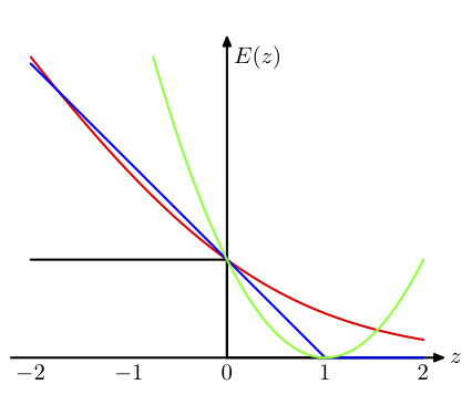
In this lecture we extended our toolbox of linear classification methods to include support vector machines (SVMs). We began with a unifying view of loss functions for classification, including squared, logistic, and misclassification loss. We then introduced the perceptron loss as a relaxation of misclassification error and discussed Rosenblatt’s perceptron algorithm. We concluded with an introduction to maximum margin classifiers and showed that the SVM optimization problem is equivalent to minimizing hinge loss with L2 regularization. See Chapters 4 and 7 of Bishop, as well as Section 4.5 and Chapter 12 of Hastie, for more detail.

Some notes:

• Coding our outcomes for binary classification as \( y_i \in
  \{-1,1\} \), we can rewrite squared and log loss as
  $$
  \mathcal{L}_{\mathrm{squared}} = \sum_i (1 – y_i \hat{y_i})^2
  $$
  and
  $$
  \mathcal{L}_{\mathrm{log}} = – \sum_i \log (1 + e^{-y_i \hat{y_i}}),
  $$
  where \( \hat{y_i} \) is the predicted label.
• Misclassification loss, on the other hand, simply incurs a cost of 1 when the signs of predicted and actual labels differ, and no cost when they agree:
  $$
  \mathcal{L}_{\mathrm{misclass}} = \sum_i \Theta( -y_i \hat{y_i} ).
  $$
  While simple to calculate, misclassification error is, unfortunately, difficult to optimize due to the discontinuity at the origin. Comparing these, we see that squared and log loss penalize incorrect predictions more heavily than misclassification error, and squared loss heavily penalizes “obviously correct” answers where the predicted and actual labels are of the same sign, but the prediction is greater that 1.
• The perceptron loss can be viewed as a relaxation of misclassification error, where correctly classified examples aren’t penalized at all and the cost of misclassification is linear in the predicted label:
  $$
  \mathcal{L}_{\mathrm{percep}} =~ – \sum_{\{i | y_i \hat{y_i} < 0\}} y_i \hat{y_i}.
  $$Following Rosenblatt’s original treatment of the perceptron leads to a simple stochastic gradient descent algorithm for minimizing this loss wherein we iteratively update our weight vector in the direction of misclassified examples. Unfortunately, even for linearly separable training data, the perceptron algorithm may converge slowly and the final solution depends on the order in which training examples are visited. Furthermore, the resulting boundary may lie close to training examples, increasing our risk of misclassifying future examples.
• We can avoid this last issue by instead searching for a maximum margin classifier—that is, we look for the boundary which is as far as possible from all training points. A bit of linear algebra reveals that we can phrase this minimization problem as:
  $$
  \mathrm{min}_{w, w_0} {1 \over 2} ||w||^2 \\
  \textrm{subject to}~ y_i(w \cdot x_i + w_0) \ge 1
  $$
  for all points \(i\), where the constraint simply states that all points are correctly classified. Intuitively we can interpret this as searching for the orientation of the thickest wedge that fits between the positive and negative classes. For small-scale problems we can use standard quadratic programming solvers to find the optimal weight vector \( w \) and bias \( w_0 \) that satisfy the above.
• The dual formulation of the problem both provides further insight into the underlying loss function and structure of SVM solutions. Specifically, one can show that SVMs minimize the hinge loss with L2 regularization:
  $$
  \mathcal{L}_{\mathrm{svm}} =~ \sum_i [1 - y_i \hat{y_i}]_+ + \lambda ||w||^2,
  $$
  where \( [ \cdot ]_+ \) indicates the positive part of the argument. This corresponds to a shifted version of the perceptron loss, where instead of paying no cost when the predicted and actual values have the same sign, correct predictions are penalized slightly if they’re too close to the boundary. Appendix E of Bishop nicely details Lagrange multipliers for inequality constraints, along with the KKT conditions, which lead to the above interpretation.
• Finally, by invoking the representer theorem and decomposing the weight vector as a linear combination of training examples \( w = \Phi^T a \), we see that SVM solutions are typically sparse in this space due to the KKT conditions. That is, most of the \( a_i \) are zero, with the non-zero multipliers corresponding exactly to the “support vectors” that serve to define the boundary.

The figure below, plagiarized from Chapter 7 of Bishop, nicely summarizes the various loss functions discussed above. In short, there are many ways of quantifying what we mean by a “good” linear predictor, and different choices lead to different types of solutions. SVMs are particularly interesting as they have a number of practical and theoretical properties of interest, most of which we haven’t discussed here. For a more detail comparison of various loss functions and their relative performance, see also Ryan Rifkin’s thesis, “Everything Old is New Again: A Fresh Look at Historical Approaches in Machine Learning.

In the second half of class we covered an introduction to MapReduce and specifically Hadoop, an open source framework for efficient parallel data processing. See the slides, borrowed from a previous tutorial, below.